The question, methods & findings
Project overview
I examined whether the twelve-item Consideration of Future Consequences scale was better described by one factor or two. I used an Open-Source Psychometrics course subset of 5,525 respondents aged 13–19, collected in 2011–2012. I fitted confirmatory factor models with FIML and tested measurement invariance across gender groups. In my original report, the two-factor model had CFI = 0.951 and RMSEA = 0.058, compared with 0.912 and 0.077 for one factor.
Results
| Model | CFI | RMSEA | AIC |
|---|---|---|---|
| One factor | 0.912 | 0.077 | 196,367 |
| Two correlated factors | 0.951 | 0.058 | 195,576 |
I transcribed the original fit statistics into original_model_fit.csv. The two factors represent prospective and immediate consequences. I also reported scalar invariance across gender groups. I have not rerun these models because the exact course data are not included.
Limitations
The smallest gender subgroup contained 77 respondents, which limits precision for its estimates and comparisons. FIML relies on a missing-at-random assumption that I did not verify. The observational sample does not support causal explanations of gender differences.
Credits
This was completed by Laura Maria Fetz. The questionnaire data came from the Open-Source Psychometrics Project.
From the project documentation. Download the overview.
The full study
Original report
Original coursework report, with its text, figures, result tables, and references. The overview above summarises the same original analysis.
Que sera, sera: Exploring Gender Identity Dynamics in Teenagers’ Consideration of Future Consequences.
Young people have perpetually wondered about the mysteries of the future. While some navigate their lives deeply considering future consequences (CFC) and meticulously plan each step, others are more akin to Doris Day’s sentiments: “Whatever will be, will be”. Previous research has shown that an individual’s CFC (i.e., the extent to which people consider the potential positive or negative outcomes of their current behavior and the level to which this consideration influences their current behavior) has implications for their health and well-being (Guo et al., 2023; Murphy & Dockray, 2018). However, whether there is a gender-specific difference in CFC is unclear. While some scholars report that men score significantly higher, suggesting that men consider the future consequences of their behavior to be more important than women do (Robbins & Burleson, 2015), others report no significant difference between males and females (Rappange et al., 2009).
In addition, it is unclear whether CFC is best explained using a single common factor or two common factors. While some scholars report satisfactory fit indices for a single-factor model (Crockett et al., 2009; Hevey et al., 2010), others report a superior fit of a two-factor model, comprising prospective CFC and immediate CFC (Rappange et al., 2009; McKay et al., 2016; Vilar et al., 2020).
Therefore, our first research aim is to investigate the dimensions of CFC. We want to probe whether the traditional one-factor model adequately explains the nature of CFC or whether a more nuanced (two-factor model) is needed, which distinguishes between prospective CFC and immediate CFC.
Next, we want to analyze whether measurement invariance can be established across different gender identities. In other words, we aim to analyze the degree to which the underlying measurement structure of CFC remains consistent or equivalent across different gender identities.
Our final research aim is then to explore the relationship between CFC and gender identity, recognizing the evolving understanding that gender identity is not solely binary. We aim to investigate potential variations in CFC among individuals identifying as boys, girls, and those with diverse gender identities. Based on our understanding of shifting gender norms and roles, we expect that the differences in consideration of future consequences (CFC) between genders may be non-existent.
Data and Participants
The data for this study is a subset of the data collected by the open-source psychometrics project between 2011 and 2012. It consists of 5525 observations from teenagers aged 13-19 years old (M = 16.72, SD = 1.64) from 111 different countries. A correlation matrix is provided in Table 1 in the Appendix. The majority of the participants were from the United States (56%), followed by Great Britain (9%), Canada (5%), and Australia (5%). Most participants identified as female (n = 3145; 57%) or male (n = 2279; 41%), while 77 participants (1%) stated they identified as neither female nor male. An overview of the percentage of participants per continent of origin and gender identity can be seen in Figure 1.
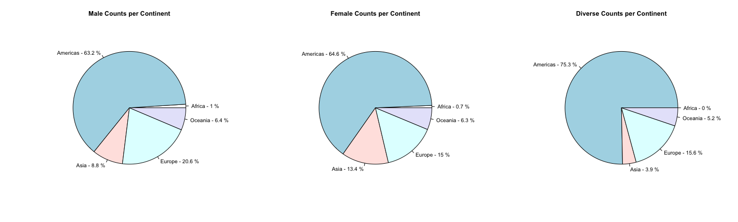
Note: Overview of the percentage of participants per continent and per gender identity.
Methods
To assess the extent to which individuals consider the potential future outcomes of their current behavior, we employed the Consideration of Future Consequences (CFC) Scale developed by Strathman et al. (1994). This instrument comprises 12 items rated on a 5-point Likert scale, ranging from "extremely uncharacteristic" (1) to "extremely characteristic" (5) of the respondent. The CFC Scale has been extensively utilized in various research contexts and has consistently demonstrated robust psychometric properties. It exhibits high internal consistency, with Cronbach's alpha typically exceeding 0.70, indicating reliable inter-item correlations (She et al., 2021).
Before our analysis, we recoded 7 of the 12 items as they were negatively worded (see CFC Questionnaire Appendix) and mean-centered all items to aid later interpretation. As our analysis was performed on raw data, we identified the degree of missingness within our data before our analysis (see Figure 2). We found that the gender variable had the highest percentage of missingness (43%). The country variable, as well as the age variable, were complete. The degree of missingness in the continent variable (given no missingness in the country variable) is to be explained by us calculating this variable using the countrycode package (v. 1.5.0; Arel-Bundock et al., 2018). While all participants indicated a country, not all country ISO values could be identified by the used package.
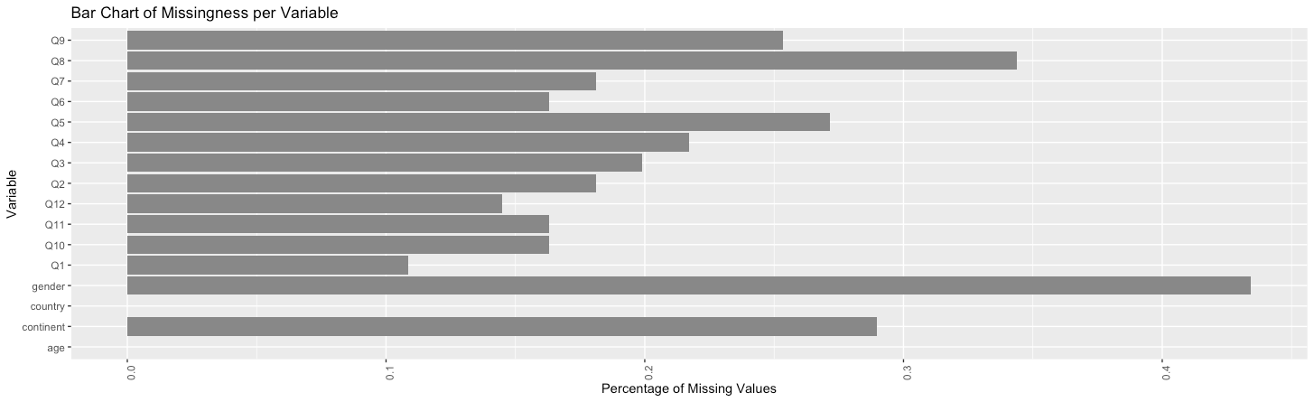
Note: The degree of missingness in the continent variable is to be explained by not all countries uniquely matching a value in the countrycode package.
Analysis
In our study, we employed Structural Equation Modeling (SEM) for Multiple Groups to examine the intricate relationships among latent variables, specifically focusing on the dimensions of Consideration of Future Consequences (CFC) and their associations with gender identity. SEM was chosen for its ability to model complex causal relationships and handle multiple regression equations simultaneously, making it ideal for our multifaceted research aims.
We conducted our analysis using R (version 4.3.0; R Core Team, 2011). The Lavaan package (version 0.6.16; Rosseel, 2012) was instrumental for performing SEM, while the semTools package (version 0.5.6; Jorgensen et al., 2020) aided in advanced model testing. For data manipulation, we relied on the Tidyverse (version 2.0.0; Wickham et al., 2019) and dplyr (version 1.1.2; Wickham et al., 2023) libraries. The psych package (version 2.3.3, Makowski, 2018) was used for descriptive statistics, and the haven library (version 2.5.2; Wickham & Miller, 2020) facilitated data importation. The semPlot (version 1.1.6.; Epskamp, 2015) and ggplot2 (version 3.4.2.; Wickham, 2016) packages were crucial for creating clear and informative visualizations.
To address missing data, we opted for Full Information Maximum Likelihood (FIML), known for its efficacy in producing unbiased parameter estimates and retaining statistical power. This method is particularly beneficial for our dataset, where missingness was present but not extensive. The optimization method used in our analysis was Nonlinear Models with Bounds (NLMINB). We used the Univariate Variance Identification (UVI) constraint for model identification, fixing the common factor variance to one. This decision was made to simplify the model structure without compromising the integrity of our estimates. We report standardized estimates, which offer intuitive interpretations akin to Pearson correlation coefficients, following Cohen’s (1992) guidelines for effect size interpretation: negligible < 0.1, ≤ small < 0.3 ≤ moderate < 0.5 ≤ large.
Model fit was assessed using the chi-square test of exact fit, root mean square error of approximation (RMSEA), and comparative fit index (CFI).
The chi-square test of exact fit measures the extent to which the predicted covariance matrix of the model matches the observed covariance matrix of the population. This test assumes that exact fit exists in the population. That is, under this null hypothesis, the associated p-value indicates the probability that the difference between the sample covariance matrix and the population covariance matrix is due to random sampling error alone. In this context, observing a significant p-value means that we reject the null hypothesis of exact fit and conclude that the model does not hold in the population. Since an exact fit is uncommon in practical applications and the chi-square test for exact fit doesn't account for sample size, we employed fit indices to assess our model. These indices served as our main criteria for determining satisfactory performance.
We used the Root Mean Square Error of Approximation (RMSEA) with a 90% confidence interval. While the chi-square test of exact fit tests whether the covariance of the population matches the observed covariance of the model, the RMSEA measures whether the covariance of the population approaches the observed covariance of the model. RMSEA values above .10 indicate a ‘poor’ fit (Brown & Cudeck, 1992), values between .08-.10 indicate a mediocre fit (MacCallum et al., 1996), while values below .05 indicate a ‘close fit’ (Brown & Cudeck, 1992). We also used the Comparative Fit Index (CFI) as an incremental fit index that compares the model of interest to a baseline model, where the population covariance is assumed to be zero. CFI > .95 indicates a good fit (Hu & Bentler, 1999).
In our analysis, we considered the model fit acceptable if the Comparative Fit Index (CFI) was good and the Root Mean Square Error of Approximation (RMSEA) fell within the acceptable range (<.10). If these conditions were not met, we refined our model by utilizing modification indices and analyzing correlation residuals. Specifically, we focused on addressing correlation residuals that exceeded .10.
To ascertain the sensitivity of our model to detect an adequate fit, we conducted an RMSEA-based power analysis using the "power4SEM" Shiny app (Jak et al., 2021). This approach, rooted in MacCallum et al. (1996), helps in evaluating if our model could reliably identify if close fit can be rejected.
To analyze whether a one-common-factor model fit the data better or if a two-common-factor model is to be preferred, we used the chi-squared difference test to compare both models as they are nested. This tests the null hypothesis that there is no difference in the model fit between the two models beyond random variability or sampling error. Therefore, a significant p-value in this context means that there is a significant difference in the model fit. We further reported the Akaike Information Criterion (AIC) as a comparative index, for which lower values generally imply a better fit.
Additionally, we tested whether measurement invariance holds to ensure that our model's factor structure was consistent across different gender identities. This involved comparing a configural model (without constraints) with a metric model (factor loadings constrained to be equal across groups), and then with a scalar model (additional constraints on intercepts). For this comparison, we also used the chi-square difference test, as these models are also nested.
Results One Factor Model
We first tested the one-factor model of CFC, where all 12 items of the CFC scale were assumed to load on a single common factor. This model can be seen in Figure 3 and is identified under the degree of freedom rule (necessary condition) (df = 162), which postulates that this model has non-negative degrees of freedom if the number of observed parameters (in this model: 270 parameters) is greater than or equal to the number of parameters to be estimated (in this model: 108 parameters). Further, this model is identified by the 3-indicator rule which is a sufficient condition, that states that each latent variable in the model must have at least three indicators to ensure proper identification, which is the case in our model.
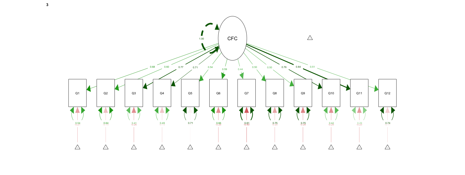
Note: The common factor variance is fixed to one as we used the UVI constraint for identification.
Despite meeting these conditions, the one-factor model demonstrated a poor fit to the data: significant chi-square test of exact fit, χ2 (162) = 1945.13, p <.001, a high AIC = 196367 and a low CFI (CFI = 0.912). In addition, RMSEA indicated a reasonable error of approximation (RMSEA = 0.077, 90% CI [0.074; 0.081]). These results suggest that the one-factor model does not adequately capture the nature and structure of CFC, and that a more nuanced model is needed.
Results Two Factor Model
Subsequently, we examined the two-factor model, dividing the CFC scale items into Immediate CFC (ICFC) and Prospective CFC (PCFC) factors. This model can be seen in Figure 4 and is identified under the degree of freedom rule (df = 159) and the 3-indicator rule. Therefore, meeting a necessary and a sufficient condition for identification
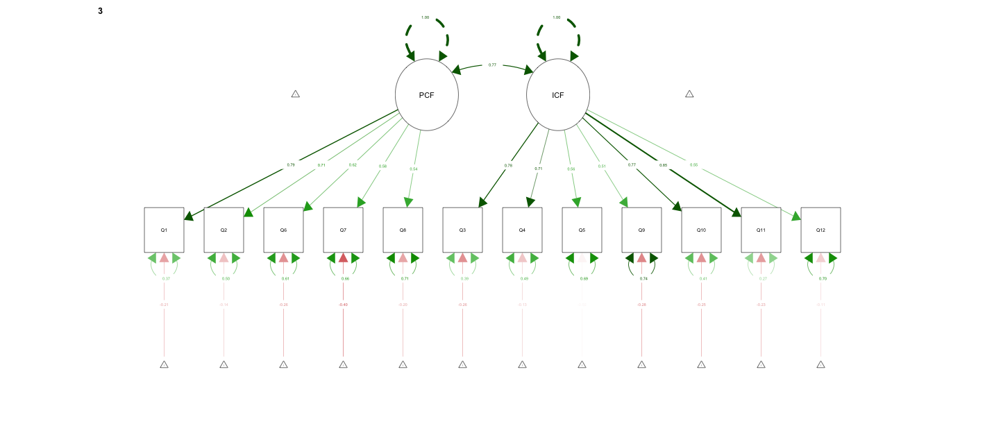
Note: The common factor variance is fixed to one as we used the UVI constraint for identification.
The two-factor model of CFC demonstrated a notably improved fit to the data compared to the one-factor model, χ2 (3) = 797.08, p <.001, ΔRMSEA = 0.381.
Although the chi-square test indicated a significant result, χ2 (159) = 1148.04, p <.001, suggesting some discrepancies, the AIC reduced (AIC = 195576), and the CFI increased to 0.951. The RMSEA improved to 0.058 (90% CI [0.055; 0.061]), falling within an acceptable range and therefore matching our criteria for accepting this model fit and test for measurement invariance.
Results Measurement Invariance
In our measurement invariance testing across gender identities, we compared configural, metric, and scalar models. The configural two-factor model, equivalent to the two-factor model mentioned above, demonstrated an acceptable fit: CFI = 0.951 and RMSEA = 0.058 (90% CI [0.055; 0.061]).
The metric model, imposing equal factor loadings across groups, also showed an acceptable fit, χ2 (179) = 1166.00, p <.001, AIC = 195554, CFI = 0.951, RMSEA = 0.055, 90% CI [0.052; 0.058] and is not significantly different to the configural model, as indicated by the non-significant chi-square difference test, Δχ2 (20) = 17.96, p = .590, ΔRMSEA = 0.00.
Similarly, the scalar model, adding constraints to factor loadings and item intercepts, maintained an acceptable fit, χ2 (199) = 1192.26, p <.001, AIC = 195540, CFI = 0.951, RMSEA = 0.052, 90% CI [0.049; 0.055]. Further, the chi-square difference test, Δχ2 (20) = 26.26, p = .156, ΔRMSEA = 0.013 suggested no significant fit reduction compared to the metric model.
These results, summarized in Table 2, imply scalar measurement invariance of the CFC two-factor model across gender identities, allowing for meaningful group comparisons.
Model | df | AIC | χ2 | Δχ2 | ΔCFI | ΔRMSEA | Δdf | p(χ2) |
|---|---|---|---|---|---|---|---|---|
Configural Model | 159 | 195576 | 1148 | |||||
Metric Model | 179 | 195554 | 1166 | 17.96 | 0.00 | 0.00 | 20 | 0.59 |
Scalar Model | 199 | 195540 | 1192 | 26.26 | 0.00 | 0.01 | 20 | 0.16 |
Scroll the table to see all columns.
Note: Strict measurement invariance was not tested, as it is not a necessary condition to compare means. The Δχ2, ΔCFI, ΔRMSEA refer to the model above respectively.
Final Model – Scalar Model
The scalar model, as our final model, showed that while there were no significant differences between boys and girls, individuals with diverse gender identities scored significantly lower on both PCFC, = -0.35, p = .010 and ICFC, = -0.28, p = .022 compared to boys.
The standardized factor loadings () indicated moderate to large associations with the common factors, detailed in Table 3.
PCAT item | Factor Loadings per Group | ||
|---|---|---|---|
1 | 2 | 3 | |
Factor 1: PCFC | |||
Q1. I consider how things might be in the future and try to influence those things with my day-to-day behavior. | 0.71 | 0.68 | 0.78 |
Q2. Often, I engage in a particular behavior in order to achieve outcomes that may not result for many years. | 0.64 | 0.61 | 0.69 |
Q6. I am willing to sacrifice my immediate happiness or well-being in order to achieve future outcomes. | 0.61 | 0.56 | 0.64 |
Q7. I think it is important to take warnings about negative outcomes seriously even if the negative outcome will not occur for many years. | 0.56 | 0.54 | 0.59 |
Q8. I think it is more important to perform a behavior with important distant consequences than a behavior with less-important immediate consequences. | 0.49 | 0.47 | 0.55 |
Factor 2: ICFC | |||
Q3. I only act to satisfy immediate concerns, figuring the future will take care of itself. | 0.78 | 0.74 | 0.80 |
Q4. My behavior is only influenced by the immediate (i.e., a matter of days or weeks) outcomes of my actions. | 0.71 | 0.68 | 0.72 |
Q5. My convenience is a big factor in the decisions I make or the actions I take. | 0.43 | 0.40 | 0.44 |
Q9. I generally ignore warnings about possible future problems because I think the problems will be resolved before they reach crisis level. | 0.63 | 0.61 | 0.63 |
Q10. I think that sacrificing now is usually unnecessary since future outcomes can be dealt with at a later time. | 0.70 | 0.68 | 0.74 |
Q11. I only act to satisfy immediate concerns, figuring that I will take care of future problems that may occur at a later date. | 0.80 | 0.79 | 0.84 |
Q12. Since my day-to-day work has specific outcomes, it is more important to me than behavior that has distant outcomes | 0.47 | 0.47 | 0.53 |
Scroll the table to see all columns.
Note: Unstandardized factor loadings are equivalent across groups. All factor loadings were significant and are hence printed in bold.
Some observed intercepts () were significant, particularly in the diverse gender identity group, denoting notable differences in response patterns. The residual variances (which can be interpreted as the variance that is not explained by the model showed great variability, ranging from 0.30 to 0.80 for the standardized estimates, indicating that there may be other factors playing a role in teenagers' answers to certain questions. The common factors () were strongly positively correlated, and the R² values (i.e. the proportion of variance explained by the factor) ranged from 0.19 to 0.80, aligning with the factor loadings. A comprehensive overview of all parameters estimates of the final model is available in Appendix Table 4.
To evaluate the robustness of our model's fit, we conducted an RMSEA-based power analysis using the "power4SEM" Shiny app. This analysis revealed that our model had a power of 1.0 to detect if a close fit can be rejected for those identifying as male or female. However, the power for the non-binary group was slightly lower at 0.75, suggesting a reduced ability to detect a close fit in this subgroup. This finding underscores the need for a cautious interpretation of the model fit in relation to the non-binary group.
Conclusion
This study explored how teenagers’ Consideration of future consequences (CFC) differs in the light of gender identities. The findings represent a nuanced understanding of CFC, highlighting the limitations of a single-factor approach and stressing the importance of adopting a more refined two-factor model, differentiating immediate CFC (ICFC) from prospective CFC (PCFC).
Moreover, this research addressed the often neglected aspect of gender identity, acknowledging the diversity that extends beyond conventional binary classifications. While those who identified as female or male exhibited similar levels of CFC, individuals with diverse gender identities showed discernible differences, indicating lower levels of both immediate and prospective CFC compared to boys. However, given the reduced power for this sample and the limited sample size, these results have to be interpreted with caution. Further crucial for the interpretation of our findings is the prevalence of missing gender variable data, which raises intriguing questions about reporting tendencies among specific gender identity groups. Are those who identify as neither female nor male perhaps more likely to report missing results on gender variables? And if so: does the likelihood depend on the country context?
Moving forward, future research should aim not only to validate our findings but also to delve deeper into the intricate interplay between gender identity and CFC and explore potential reasons behind missing data in certain gender identity groups. This could enrich our understanding. Moreover, advocating for larger and more diverse samples would enhance the robustness and applicability of subsequent studies in this realm.
Overall, this study contributes to the need for broader conversations on gender diversity, prompting a reevaluation of conventional perspectives on future-oriented considerations. Embracing inclusivity and further probing into these realms will not only refine our understanding but also foster equality within our society.
References:
Arel-Bundock et al., (2018). countrycode: An R package to convert country names and country codes . Journal of Open Source Software, 3(28), 848. https://doi.org/10.21105/joss.00848
Browne, M.W. and Cudeck, R. (1992) Alternative Ways of Assessing Model Fit. Sociological Methods and Research, 21, 230-258. https://doi.org/10.1177/0049124192021002005
Cohen, J. (1992). A power primer. Psychological Bulletin, 112(1), 155–159. doi:10.1037/0033- 2909.112.1.155.
Crockett, R. A., Weinman, J., Hankins, M., & Marteau, T. (2009). Time orientation and health- related behaviour: Measurement in general population samples. Psychology and Health, 24(3), 333-350.
Epskamp, S. (2015). semPlot: Unified visualizations of structural equation models. Structural Equation Modeling, 22(3), 474–483. https://doi.org/10.1080/10705511.2014.937847
Guo, M., Lou, Y. & Zhang, N. (2023). Consideration of future consequences and self-control mediate the impact of time perspectives on self-rated health and engagement in healthy lifestyles among young adults. Curr Psychol 42, 19670–19680. https://doi.org/10.1007/s12144-022-03135-6.
Hevey, D., Pertl, M., Thomas, K., Maher, L., Craig, A., & Chuinneagain, S. N. (2010). Consideration of future consequences scale: Confirmatory factor analysis. Personality and Individual Differences, 48(5), 654-657.
Hu, L.-t., & Bentler, P. M. (1999). Cutoff criteria for fit indexes in covariance structure analysis: Conventional criteria versus new alternatives. Structural Equation Modeling, 6(1), 1–55. https://doi.org/10.1080/10705519909540118
Jak, S., Jorgensen, T. D., Verdam, M. G., Oort, F. J., & Elffers, L. (2021). Analytical power calculations for structural equation modeling: A tutorial and Shiny app. Behavior Research Methods, 53, 1385-1406.
Jorgensen, T. D., Pornprasertmanit, S., Schoemann, A. M., Rosseel, Y., Miller, P., Quick, C., & Coffman, D. (2016). Package ‘semtools’. Website: https://cran. r-proje ct. org/web/packa ges/semTo ols/semTools. pdf.
MacCallum, R. C., Browne, M. W., & Sugawara, H. M. (1996). Power analysis and determination of sample size for covariance structure modeling. Psychological Methods, 1(2), 130–149. https://doi.org/10.1037/1082-989X.1.2.130
Makowski, D. (2018). The psycho package: An efficient and publishing-oriented workflow for psychological science. Journal of Open Source Software, 3(22), 470.
McKay, M. T., Perry, J. L., Percy, A., & Cole, J. C. (2016). Evidence for the reliability and validity, and some support for the practical utility of the two-factor Consideration of Future Consequences Scale-14. Personality and Individual Differences, 98, 133-136.
Murphy, L., & Dockray, S. (2018). The consideration of future consequences and health behaviour: a meta-analysis. Health psychology review, 12(4), 357–381. https://doi.org/10.1080/17437199.2018.1489298
R Development Core Team (2011) R: A language and environment for statistical computing. R Foundation for Statistical Computing, Vienna. http://www.R-project.org
Rappange, D., Werner, B.F. & Van Exel, N.J. (2009). Back to the consideration of the future consequences scale: Time to reconsider. The Journal of Social Psychology, 149(5), 562- 584.
Robbins, T., & Burleson, J. (2015). Consideration of future consequences: A closer look at gender and cultural differences. International Journal of Business and Social Science, 6(5), 1-6.
Rosseel, Y. (2012). lavaan: An R Package for Structural Equation Modeling. Journal of Statistical Software, 48(2), 1–36. https://doi.org/10.18637/jss.v048.i02
She, L., Ma, L., & Khoshnavay Fomani, F. (2021). The consideration of future consequences scale among Malaysian young adults: a psychometric evaluation. Frontiers in psychology, 12, 770609.
Strathman, A., Gleicher, F., Boninger, D. S., & Edwards, C. S. (1994). The consideration of future consequences: Weighing immediate and distant outcomes of behavior. Journal of personality and social psychology, 66(4), 742.
Tavakol, M., & Wetzel, A. (2020). Factor Analysis: a means for theory and instrument development in support of construct validity. International journal of medical education, 11, 245–247. https://doi.org/10.5116/ijme.5f96.0f4a
Vilar, R., Milfont, T. L., Araújo, R. D. C. R., Coelho, G. L. D. H., Soares, A. K. S., & Gouveia, V. V. (2020). Consideration of future consequences (CFC): Validation and proposition of an ultra-short scale. Current Psychology, 1-15.
Wickham, H., Averick, M., Bryan, J., Chang, W., McGowan, L. D. A., François, R., & Yutani, H. (2019). Welcome to the Tidyverse. Journal of open source software, 4(43), 1686.
Wickham, H. (2016). ggplot2: Elegant Graphics for Data Analysis. Springer. https://ggplot2.tidyverse.org
Wickham H, François R, Henry L, Müller K, Vaughan D (2023). dplyr: A Grammar of Data Manipulation. R package version 1.1.4. https://github.com/tidyverse/dplyr, https://dplyr.tidyverse.org.
Wickham, H., Miller, E., & Smith, D. (2020). haven: Import and Export'SPSS', 'Stata' and 'SAS' Files. R package version 2.3. 1.
Appendix
Q1 | Q2 | Q3 | Q4 | Q5 | Q6 | Q7 | Q8 | Q9 | Q10 | Q11 | Q12 | age | gender | M | SD | |
|---|---|---|---|---|---|---|---|---|---|---|---|---|---|---|---|---|
Q1 | 1.00 | 0.00 | 1.14 | |||||||||||||
Q2 | 0.49 | 1.00 | 0.00 | 1.30 | ||||||||||||
Q3 | 0.45 | 0.38 | 1.00 | 0.00 | 1.34 | |||||||||||
Q4 | 0.40 | 0.37 | 0.58 | 1.00 | 0.00 | 1.32 | ||||||||||
Q5 | 0.19 | 0.19 | 0.31 | 0.33 | 1.00 | 0.00 | 1.16 | |||||||||
Q6 | 0.38 | 0.36 | 0.36 | 0.31 | 0.22 | 1.00 | 0.00 | 1.25 | ||||||||
Q7 | 0.36 | 0.30 | 0.32 | 0.29 | 0.15 | 0.33 | 1.00 | 0.00 | 1.15 | |||||||
Q8 | 0.31 | 0.29 | 0.29 | 0.26 | 0.12 | 0.32 | 0.32 | 1.00 | 0.00 | 1.11 | ||||||
Q9 | 0.35 | 0.28 | 0.45 | 0.39 | 0.25 | 0.27 | 0.43 | 0.27 | 1.00 | 0.00 | 1.36 | |||||
Q10 | 0.37 | 0.35 | 0.48 | 0.43 | 0.28 | 0.41 | 0.34 | 0.26 | 0.48 | 1.00 | 0.00 | 1.30 | ||||
Q11 | 0.43 | 0.38 | 0.60 | 0.54 | 0.34 | 0.38 | 0.34 | 0.28 | 0.49 | 0.57 | 1.00 | 0.00 | 1.32 | |||
Q12 | 0.23 | 0.25 | 0.36 | 0.36 | 0.24 | 0.21 | 0.18 | 0.18 | 0.25 | 0.32 | 0.37 | 1.00 | 0.00 | 1.12 | ||
age | 0.00 | -0.05 | 0.01 | 0.02 | 0.01 | 0.01 | 0.00 | 0.00 | -0.01 | 0.02 | 0.01 | 0.00 | 1.00 | 16.72 | 1.64 | |
gender | 0.01 | 0.00 | -0.01 | 0.00 | 0.01 | -0.01 | -0.01 | -0.01 | 0.00 | 0.01 | -0.01 | -0.03 | -0.08 | 1.00 | 1.60 | 0.52 |
Scroll the table to see all columns.
Note: The means of the CFC Questions are zero as we mean centered them.
Factor loadings | Intercepts | Residual Variance | Common Factor Covariance | R2 | |||||||||||
|---|---|---|---|---|---|---|---|---|---|---|---|---|---|---|---|
1 | 2 | 3 | 1 | 2 | 3 | 1 | 2 | 3 | 1 | 2 | 3 | 1 | 2 | 3 | |
Q1 | 0.83 (0.71) | 0.83 (0.68) | 0.83 (0.78) | -0.00 (-0.00) | -0.00 (-0.00) | -0.00 (-0.00) | 0.69 (0.50) | 0.66 (0.54) | 0.50 (0.39) | 0.50 | 0.46 | 0.61 | |||
Q2 | 0.86 (0.64) | 0.83 (0.61) | 0.83 (0.69) | -0.00 (-0.00) | -0.00 (-0.00) | -0.00 (-0.00) | 1.04 (0.59) | 1.02 (0.63) | 0.93 (0.53) | 0.41 | 0.37 | 0.47 | |||
Q3 | 1.05 (0.78) | 1.05 (0.74) | 1.05 (0.80) | -0.00 (-0.00) | -0.00 (-0.00) | -0.00 (-0.00) | 0.69 (0.39) | 0.80 (0.45) | 0.64 (0.36) | 0.62 | 0.55 | 0.64 | |||
Q4 | 0.96 (0.71) | 0.96 (0.68) | 0.96 (0.72) | -0.00 (-0.00) | -0.00 (-0.00) | -0.00 (-0.00) | 0.89 (0.49) | 0.92 (0.54) | 0.88 (0.49) | 0.51 | 0.47 | 0.51 | |||
Q5 | 0.51 (0.43) | 0.51 (0.40) | 0.51 (0.44) | -0.00 (-0.00) | -0.00 (-0.00) | -0.00 (-0.00) | 1.10 (0.81) | 1.12 (0.83) | 1.057 (0.80) | 0.19 | 0.17 | 0.20 | |||
Q6 | 0.77 (0.61) | 0.77 (0.56) | 0.77 (0.64) | -0.00 (-0.00) | -0.00 (-0.00) | -0.00 (-0.00) | 1.00 (0.63) | 1.06 (0.68) | 0.97 (0.59) | 0.37 | 0.32 | 0.41 | |||
Q7 | 0.66 (0.56) | 0.66 (0.54) | 0.66 (0.59) | -0.00 (-0.00) | -0.00 (-0.00) | -0.00 (-0.00) | 0.98 (0.69) | 0.89 (0.71) | 0.95 (0.66) | 0.31 | 0.29 | 0.34 | |||
Q8 | 0.56 (0.49) | 0.56 (0.47) | 0.56 (0.55) | -0.00 (-0.00) | -0.00 (-0.00) | -0.00 (-0.00) | 0.99 (0.76) | 0.90 (0.78) | 0.82 (0.70) | 0.24 | 0.23 | 0.30 | |||
Q9 | 0.87 (0.63) | 0.87 (0.61) | 0.87 (0.63) | -0.00 (-0.00) | -0.00 (-0.00) | -0.00 (-0.00) | 1.16 (0.60) | 1.14 (0.63) | 1.18 (0.60) | 0.40 | 0.37 | 0.40 | |||
Q10 | 0.93 (0.70) | 0.93 (0.68) | 0.93 (0.74) | -0.00 (-0.00) | -0.00 (-0.00) | -0.00 (-0.00) | 0.90 (0.51) | 0.89 (0.54) | 0.71 (0.45) | 0.49 | 0.46 | 0.55 | |||
Q11 | 1.09 (0.80) | 1.09 (0.79) | 1.09 (0.84) | -0.00 (-0.00) | -0.00 (-0.00) | -0.00 (-0.00) | 0.65 (0.36) | 0.63 (0.38) | 0.51 (0.30) | 0.64 | 0.62 | 0.70 | |||
Q12 | 0.55 (0.47) | 0.55 (0.47) | 0.55 (0.53) | -0.00 (-0.00) | -0.00 (-0.00) | -0.00 (-0.00) | 1.05 (0.78) | 0.92 (0.78) | 0.79 (0.72) | 0.22 | 0.22 | 0.28 | |||
PCFC | 0.00 (0.00) | 0.02 (0.02) | -0.35 (-0.33) | 1.00 (1.00) | 0.83 (1.00) | 1.13 (1.00) | |||||||||
ICFC | 0.00 (0.00) | 0.01 (0.01) | -0.28 (-0.28) | 1.00 (1.00) | 0.87 (1.00) | 1.02 (1.00) | |||||||||
PCFC ~~ ICFC | 0.82 (0.82) | 0.67 (0.79) | 0.84 (0.78) | ||||||||||||
Scroll the table to see all columns.
Note: Standardized parameters are in brackets. Bold printed estimates were significant. (>.05).